Data Science meets SEO, Part 2


After I explained in the first part what data science is and what already exists in this area on the subject of SEO, now the second part, where we take a closer look at what the linguistic processing of a document by a search engine has on SEO concepts such as keyword density, TF/IDF and WDF/IDF. Since I showed Campixx live code at SEO, I offer everything for download here, which makes following the examples even more eventful. By the way, this is also possible without the installation of R, here you can find the complete code with explanations and results.

For those who want to recreate it in R

(Please skip if you don’t want to recreate this yourself in R)

I recommend using RStudio in addition to R, because handling the data is a bit easier for newbies (and for professionals as well). R is available at the R ProjectRStudio on rstudio.com. First install R, then RStudio.

In the ZIP file there are two files, a notebook and a CSV file with a small text corpus. I refer to the notebook from time to time in this text, but the notebook can also be worked through in this way. Important: Please do not read the CSV file with the import button, because then a library will be loaded, which will nullify the functionality of another library.

The notebook has the great advantage that both my description, the program code and the result can be seen in the same document.

To execute the program code, simply click on the green arrow in the upper right corner, and it works

What is TF/IDF or WDF/IDF?

(Please skip if the concepts are clear!)

There are people who can explain TF/IDF (Term Frequency/Inverse Document Frequency) or WDF/IDF (Word Document Frequency/Inverse Document Frequency) better than me, at WDF/IDF Karl has distinguished himself with an incredibly good article (and by the way, in this article he has already said that “actually no small or medium-sized provider of analysis tools can offer such a calculation for a large number of users … ; -“).

A simplistic explanation is that the term frequency (TF) is the frequency of a term in a document, while the Inverse Document Frequency (IDF) measures the importance of a term in relation to all documents in a corpus in which the term occurs (corpus is the linguists’ term for a collection of documents; this is not the same as an index).

In TF, the number of occurrences of a term is counted, simplified but still far too complicated, and then normalized, usually by dividing that number by the number of all words in the document (this definition can be found in the book “Modern Information Retrieval” by Baeza-Yates et al, the bible of search engine builders). But there are other weightings of the TF, and WDF is actually nothing more than such a different weighting, because here the term frequency is provided by a logarithm to base 2.

In the IDF, the number of all documents in the corpus is divided by the number of documents in which the term appears, and the result is then provided with a logarithm to base 2. The Term Frequency or the Word Document Frequency is then multiplied by the Inverse Document Frequency, and we have TF/IDF (or, if we used WDF instead of TF, WDF/IDF). The question that arises to me as an ex-employee of several search engines, however, is what exactly is a term here, because behind the scenes the documents are eagerly tinkered with. More on this in the next section “Crash Course Stemming…”.

Crash Course Stemming, Composite and Proximity

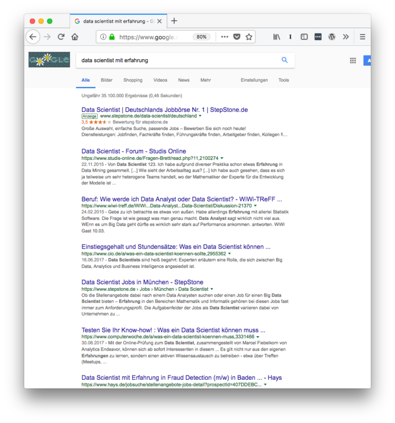
Everyone has had the experience that you search for a term and then get a results page where the term can also be found in a modified form. This is because, for example, stemming is carried out, in which words are reduced to their word stem. Because not only in German is conjugated and declined, other languages also change words depending on the person, tense, etc. In order to increase the recall, not only the exact term is searched for, but also variants of this term (I did not use the term “recall” in the lecture, it describes in the Information Retrieval how many suitable documents are found for a search query). For example, for the search query “Data scientist with experience”, documents are also found that contain the terms “data scientist” and “experience” (see screenshot on the left).

In the lecture, I “lifted” live, with the SnowballC-Stemmer. This is not necessarily the best stemmer, but it gives an impression of how stemming works. In the R-Notebook for this article, the Stemmer is slightly expanded, because unfortunately the SnowBallC only ever lifts the last word, so that the Stemmer has been packed into a function that can then handle a whole set completely:

> stem_text(“This is a great post”) [1] “This is a great post” > stem_text(“Hope you’ve read this far.”) [1] “Hopefully you have read this far.”

But they are not just variants of a term. We Germans in particular are world champions in inventing new words by “composing” them by putting them together with other words. It is not for nothing that these neologisms are called compounds. An example of the processing of compounds can be found in the screenshot on the right, where the country triangle becomes the border triangle. First of all, it sounds quite simple, you simply separate terms that could stand as a single word and then index them. However, it is not quite that simple. Because not every compound may be separated, because it takes on a different meaning separately. Think, for example, of “pressure drop”, where the drop in pressure could also be interpreted as pressure and waste

The example of the “data scientist with experience” also illustrates another method of search engines: Terms do not have to be together. They can be further apart, which can sometimes be extremely annoying for the searcher if one of the terms in the search query is in a completely different context. The proximity, i.e. the proximity of the terms, can be a signal for the relevance of the terms present in the document for the search query. Google offers Proximity as a feature, but it is not clear how Proximity will be used as a ranking signal. And this only means the textual proximity, not yet the semantic proximity. Of course, there is much more processing in lexical analysis, apart from stop word removal etc. But for now, this is just a small insight.

So we see three points here that most SEO tools can’t do: stemming, proximity and decompounding. So when you talk about keyword density, TF/IDF or WDF/IDF in the tools, it’s usually based on exact matches and not the variants that a search engine processes. This is not clear with most tools; for example, the ever-popular Yoast SEO plugin for WordPress can only use the exact match and then calculates a keyword density (number of the term in relation to all words in the document). But ryte.com says, for example:

In addition, the formula WDF*IDF alone does not take into account that search terms can also occur more frequently in a paragraph, that stemming rules could apply or that a text works more with synonyms.

So as long as SEO tools can’t do that, we can’t assume that these tools give us “real” values, and that’s exactly what dear Karl Kratz has already said. These are values that were calculated on the basis of an exact match, whereas search engines use a different basis. Maybe it doesn’t matter at all, because everyone only uses the SEO tools and optimizes for them, we’ll take a look at that in the next part. But there are other reasons why the tools don’t give us the whole view, and we’ll take a closer look at them in the next section.

Can we measure TF/IDF or WDF/IDF properly at all?

Now, the definition of IDF already says why a tool that spits out TF/IDF has a small problem: It doesn’t know how many documents with the term are in the Google corpus, unless this number is also “scraped” from the results. And here we are dealing more with estimates. It is not for nothing that the search results always say “Approximately 92,800 results”. Instead, most tools use either the top 10, the top 100, or maybe even their own small index to calculate the IDF. In addition, we also need the number of ALL documents in the Google index (or all documents of a language area, which Karl Kratz drew my attention to again). According to Google, this is 130 trillion documents. So, in a very simplified way, we would have to calculate like this (I’ll take TF/IDF, so that the logarithm doesn’t scare everyone off, but the principle is the same):

TF/IDF = (Frequency of the term in the document/Number of words in the document)*log(130 trillion/”Approximately x results”),

where x is the number that Google displays per search result. So, and then we would have one number per document, but we don’t know what TF/IDF or WDF/IDF value the documents that are not among the top 10 or top 100 results examined. It could be that there is a document in 967th place that has better values. We only see our excerpt and assume that this excerpt explains the world to us.

And this is where chaos theory comes into play: Anyone who has seen Jurassic Park (or even read the book) may remember the chaos theorist, played by Jeff Goldblum in the film. Chaos theory plays a major role in Jurassic Park, because it is about the fact that complex systems can exhibit behavior that is difficult to predict. And so large parts of the park are monitored by video cameras, except for 3% of the area, and this is exactly where the female dinosaurs reproduce. Because they can change their sex (which frogs, for example, can also do). Transferred to TF/IDF and WDF/IDF, this means: we don’t see 97% of the area, but less than 1% (the top 10 or top 100 of the search results) and don’t know what’s lying dormant in the rest of our search results page. Nevertheless, we try to predict something on the basis of this small part.

Does this mean that TF/IDF or WDF/IDF are nonsense? No, so far I have only shown that these values do not necessarily have anything to do with what values a search engine has internally. And this is not even new information, but already documented by Karl and some tool providers. Therefore, in the next part, we will take a closer look at whether or not we can find a correlation between TF/IDF or WDF/IDF and position on the search results page.

Say it with data or it didn’t happen

In the enclosed R-notebook, I have chosen an example to illustrate this, which (hopefully) reminds us all of school, namely I have made a small corpus of Goethe poems (at least here I have no copyright problems, I was not quite so sure about the search results). A little more than 100 poems, one of which I still know by heart after 30 years. In this wonderful little corpus, I first normalize all the words by lowering them all, removing numbers, removing periods, commas, etc., and removing stop words.

Although there is a library tm in R with which you can calculate TF/IDF as well as TF (normalized)/IDF, but, scandal (!!), nothing about WDF/IDF. Maybe I’ll build a package for it myself. But for illustrative purposes, I just built all the variants myself and put them next to each other. So you can see for yourself what I did in my code. Let’s take a look at the data for the unstemmed version:

We can see here that the “ranking” would change if we were to sort by TF/IDF or TF (normalized)/IDF. So there is a difference between WDF/IDF and the “classical” methods. And now let’s take a look at the data for the managed version:

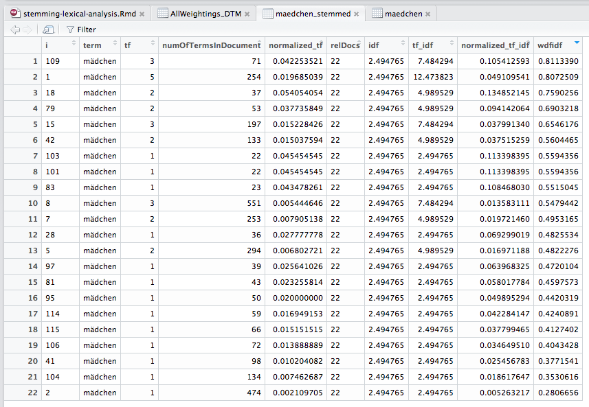
We see that two documents have cheated their way into the top 10, and also that we suddenly have 22 instead of 20 documents. This is logical, because a term with two or more different stems can now have become one. But we also see very quickly that all the numbers have changed. Because now we have a different basis. In other words, whatever SEOs read from WDF/IDF, the values are most likely not what actually happens at Google. And again: This is not news! Karl Kratz has already said this, and some tools also say this in their glossaries. After my lecture, however, it seemed as if I had said that God does not exist

And perhaps it is also the case that the rapprochement alone works. We’ll look at that in the next parts about data science and SEO.

Was that data science?

Phew. No. Not really. Just because you’re working with R doesn’t mean you’re doing data science. But at least we warmed up a bit by really understanding how our tool actually works.

Data Science meets SEO, Part 1


On 1.3.2018 I gave a lecture on the topic of data science and SEO at the SEO Campixx, and since there were some discussions afterwards :-), I will describe the contents in more detail here, in several parts. This part is first of all about what data science is and what already exists on the topic.

What exactly is data science?

The sexiest job of the 21st century” is rather dull on closer inspection, because most of the time is spent acquiring and cleaning data and using it to build models. It’s coding, it’s math, it’s statistics, and with larger amounts of data, it’s also a lot of knowledge about where to wire which instances with each other, such as on Amazon Web Services or Google Cloud Platform. A global galactic definition of data science does not exist to my knowledge, but I would consider data science to be the intersection of

  • Data Mining
  • Statistics and
  • Machine Learning

define. These are not new topics, but what is new is that we have much more data, much faster processors, cheap cloud processing and many development libraries. For the statistics language and development environment R used here, libraries exist for almost every purpose; somewhere there was someone who was faced with the same problem and then built a solution for it. What is also new is that more and more companies feel that you can do something with data, after all, Spotify uses data to know what music you might still like, and Google knows when you should set off if you want to get to work on time.

Unfortunately, the data hype (which will be followed by a healthy understanding of what is possible after a plateau of disappointment) is countered by relatively few people who feel at home in all three disciplines (plus cloud computing). Which in turn leads to the fact that these data scientist unicorns are sometimes offered unreasonable sums and 1000s of courses are offered on Udemy & Co that are supposed to provide you with the necessary knowledge.

A real problem with data science, however, is that not only knowledge in several areas is necessary, but also the understanding that data is used to solve a problem. I can deal with algorithms and data all day long, for me it’s like a kind of meditation and relaxation. In fact, sometimes I feel like playing with Lego, but at the end of the day, it’s all about solving problems. Not only collecting data, but also extracting the right information from it and then taking the right action (the holy trinity of data). And here is the challenge that often enough people just say, here is data, make something out of it. Therefore, it is an art for the data scientist to understand exactly what the problem actually is and to translate this into code.

In addition, many people have bad memories of math. Accordingly, the audience’s willingness to consume slides with lots of numbers and formulas tends to be on the lower end of the scale. That’s why I also worked with smaller examples in the lecture, which everyone should be able to understand well.

What kind of topics am I working on? Very different. Classification. Clustering. Personalization. Chatbots. But also analyses of slightly larger data volumes of 25 million rows of Analytics data and more, which have to be processed in a few minutes. All kinds of things.

What is already there?

On the search engine side, there is already a lot. When I was still at Ask, we had already worked with Support Vector Machines, for example, to create the ranking for the queries where the pages had almost no backlinks. Even then, there was a dynamic ranking. The topic recognition of most search engines is based on machine learning. RankBrain will be based on machine learning. So it’s not a new topic for search engines.

On the other hand, that of SEOs, the topic still seems to be relatively fresh. Search Engine Land says thatevery search marketer can think of themselves as a data scientist. I’m not sure I would subscribe to that, because most search marketers I know don’t build their own models. As a rule, they use tools that do this for them. On SEMRush you can find a collection of ideas, but more for SEA. Remi Bacha is still exciting, although I haven’t seen any data from him yet. Keyword Hero have come up with something pretty cool by using deep learning to identify the organic keywords that are no longer included since the switch to https. Otherwise, I haven’t seen much on the subject. So we see that we are at the very beginning.

What would we like to have?

Back to the question of what problem I actually want to solve with my work. In an ideal world, SEO naturally wants to be able to re-engineer the Google algorithm. However, this is unlikely, because of the more than 200 ranking signals, only a few are available to us. What we can do, however, is try to build models with the signals we have, and possibly create smaller tools. And that’s exactly what the next part is about

Why the average session duration in Analytics is complete nonsense


I have been dealing with web analysis for over 20 years, starting with server log files and today with sometimes crazy implementations of tracking systems. The possibilities are getting better and better, but not everything has gotten better. Because one superstition simply cannot be killed, namely that Time on Site or the “average session duration” is a good metric, or that the given values are correct at all, so here is black and white: In a standard implementation, the Time on Site is not measured correctly, whether in Adobe Analytics or Google Analytics or Piwik or whatever.

Why Average Session Duration Isn’t Measured Properly

The explanation why the times cannot be correct is quite simple. In a standard installation of Google/Adobe Analytics/[place your system here], a measurement is performed every time the user triggers an action. For example, it comes to a website at 1:00 p.m., and then the tracking pixel is triggered for the first time. The user looks around a bit and then clicks on a link at 1:01 p.m., so that he gets to another page of the same website, where the tracking pixel is fired again. Now we can calculate that he has spent 1 minute on the website so far, because we have two measurement points with different timestamps. We measure time here with the temporal distance between two sides.

On the second page, on which he is now located, the user stays longer, because here he finds what he was looking for. He reads a text, and at 1:05 p.m., i.e. after 4 minutes, his need for information is satisfied, so he leaves the page. So he was now on the website for a total of 5 minutes. However, Analytics only knows about the 1st minute and will only include this 1 minute in the statistics. Because when you leave the page, nothing is fired. As written above: We measure time with the time distance between two pages. Time distance between 1st and 2nd page: 1 minute. Temporal distance between 2nd and exit: Not measurable, because the next page is missing. And most users are not aware of this. The time a user spends on the last page is not measured.

Can’t Analytics measure when a user leaves the page? No, it can’t, no matter which system. At least not in the standard installation. Of course, these can be adjusted. Otherwise: If a user comes to a website and only looks at one page, then no time is measured. Even if he spends 10 minutes on this one side, it does not flow into the average session duration. Since a one-page visit is not uncommon, quite a lot of data is missing.

Is that really that bad?

Does that really make that much difference? Yes, it does. It is often said of the astonished user that with the figures given, one would at least have a clue. What can you do with a clue that is completely wrong? Of course, no one likes to admit that all previous data was wrong and so were the decisions based on it.

To illustrate the differences, here are a few data points. Until August 2017, the average session duration on my site was 1 minute on average (red line, here compared to the previous year). As of August 2017, the average session duration increases to 5 minutes (blue line). The time on site has increased fivefold and also seems much more realistic, since most of the content on my site cannot be read in 1 minute. However, even these 5 minutes are not the actual average session time, but only an approximation.

How do you get better figures?

How is it that more of time is now being measured? In another article I had written about measuring the scroll depth, and here an event is fired when reaching 25%, 50%, 75% and 100% of the page length. With each of these events, a timestamp is also sent. If a user scrolls down, a period of time is also measured from the last page of a visit, until the last event is triggered. It’s not unlikely that users will spend even more time on this page, as they may read something in the bottom section but stop scrolling.

Why, the question could now be, isn’t an event simply triggered every second as long as the user is on the site? Then you would have an exact duration of the meeting. Technically, this is actually possible, but with Google Analytics, for example, the free version allows a maximum of 10 million hits per month (hit = server call), with Adobe every single hit is billed. So I should allow myself 333,333 hits per day with Google Analytics, and if we assume an actual average session duration of 6 minutes (360 seconds), then I should have less than 1,000 users per day, so that I don’t get the juice turned off. And we haven’t measured anything else with that. Even with the scroll depth measurement, so many server calls would already be triggered on many pages that you simply can’t afford it. Here, however, at least a random sample of users can be measured in order to at least get an approximation worthy of the name.

Why use the average session duration at all?

This metric is often used when there are no “hard” conversions, for example when awareness is one of the marketing goals and only users should initially come to the site. But maybe a lot of time is only wasted because the desired information is not found, but urgently needed (have you ever looked for a driver on hp.com?); in other words, maybe a shorter time is even better?

As always, it’s a question of how well segmenting is done. For hp.com, a metric like “time to download” would be good, for a content-only page, the scroll depth paired with the time spent on the page would be a good indicator of how well the content is interacted. In addition, it would be necessary to take into account how much content is available on a page. This can be done with Custom Dimensions, for example. My favorite saying: Every minute that a user spends on my customer’s site, he cannot spend on the website of his market competitor.

However, the real average session duration is also exciting because the concept of holistic landing pages is drawing ever wider circles. Since Google sometimes also receives signals about how long someone has been on a page (for example, by returning to a search results page), every search engine optimizer should also be interested in how long someone was actually on a page and which parts of the holistic content were actually read (after all, the content is written for users and not for GoogleBot… or?

Result

The average session duration or time on site in any analytics system provides incorrect numbers in a standard installation, which is clear to very few users. This can be remedied by triggering events, for example for scroll tracking. As is so often the case: A Fool with a Tool is still a Fool. As long as you don’t deal with how a tool measures something, you shouldn’t be surprised if the conclusions drawn from it are wrong. This applies to analytics as well as to Google Trends or Similar Web

Linear regression: How much can a used SLR camera cost?


Since the Canon 5d Mark IV has just been released, the 5d Mark III will also be affordable. I was advised to pay €1,500 for a maximum of 30,000 releases, but if you look at the cameras on offer on eBay and the relevant forums, the price seems to be much higher. But what is the fair price? With sufficient data, this can be determined by regression.

First of all, let’s assume that the more shutter releases a camera has, the cheaper it becomes. 150,000 triggers is the expected life of the shutter release on the 5d Mark III, a new shutter release including labor costs about 450€ (not verified). But first, let’s take a look at what the data looks like. I have picked out the prices and releases of almost 30 offers from the various platforms, so this does not take into account how good the camera is on the outside or what accessories are included. This data is read into R and examined for its characteristics:

We have an average price of 1,666€ and an average number of triggers of 85,891. That’s a far from the €1,500 with 30,000 triggers. The median does not look much better either. Now we start the regression and form a regression model with the function lm and look at the details with the command summary(MODELNAME):

From this we can already form a function:

Price = -0.001749x+1816 where x is the number of triggers. So a camera with 30,000 shutters should cost €1,763.53, a camera with 100,000 shutters still €1,614. Let’s take a look at the plot:

As you can see, we have some outliers (by the way, not due to great accessories or maintenance etc.) that somewhat “distort” the model. I had already removed a camera with nearly 400,000 releases and a price of still €1,000.

Unfortunately, the number of triggers cannot be automatically read from the portals because it is always manually entered by the user. Otherwise, you could build a nice tool for each camera model.